SURF Feature Descriptors on Python OpenCV

This entry is part 1 of 1 in the series Image Feature Descriptors

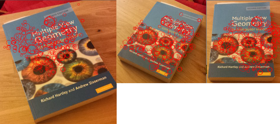
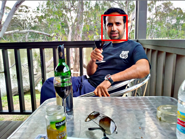
This is a test of SURF features (http://en.wikipedia.org/wiki/SURF, claimed to be faster than the original SIFT feature descriptors) on Python OpenCV.
Parameters used were: (0, 300, 3, 4)
0: (basic, 64-element feature descriptors)
hessian threshold: 300
number of octaves: 3
number of layers within each octave: 4
Time taken for execution: 0.108652 seconds on a 249×306 image (MacBook Air 2.13 GhZ, Core 2 Duo, 4 GB RAM)


import cv

# SURF Feature Descriptor
# 
# Programmed by Jay Chakravarty


import cv
from time import time

    
if __name__ == '__main__':
    cv_image1=cv.LoadImageM("mvg1.jpg")
    cv_image2=cv.LoadImageM("mvg2.jpg")
    cv_image1_grey = cv.CreateImage( (cv_image1.width, cv_image1.height), 8, 1 )
    cv.Zero(cv_image1_grey)
    cv_image2_grey = cv.CreateImage( (cv_image2.width, cv_image2.height), 8, 1 )
    cv.Zero(cv_image2_grey)

    #cv.ShowImage("mvg1", cv_image1)
    #cv.ShowImage("mvg2", cv_image2)  
    cv.CvtColor(cv_image1, cv_image1_grey, cv.CV_BGR2GRAY);
    #cv.ShowImage("mvg1_grey", cv_image1_grey)  
    cv.CvtColor(cv_image2, cv_image2_grey, cv.CV_BGR2GRAY);
    #cv.ShowImage("mvg2_grey", cv_image2_grey);
    
    #CvSeq *imageKeypoints = 0, *imageDescriptors = 0;
    
    # SURF descriptors
    #param1: extended: 0 means basic descriptors (64 elements each), 1 means extended descriptors (128 elements each)
    #param2: hessianThreshold: only features with hessian larger than that are extracted. good default value is 
    #~300-500 (can depend on the average local contrast and sharpness of the image). user can further filter out
    #some features based on their hessian values and other characteristics.
    #param3: nOctaves the number of octaves to be used for extraction. With each next octave the feature size is
    # doubled (3 by default)
    #param4: nOctaveLayers The number of layers within each octave (4 by default)
    
    tt = float(time())    

    #SURF for image1
    (keypoints1, descriptors1) = cv.ExtractSURF(cv_image1_grey, None, cv.CreateMemStorage(), (0, 300, 3, 4))
    
    tt = float(time()) - tt
    
    print("SURF time image 1 = %g seconds\n" % (tt))
    
    #print "num of keypoints: %d" % len(keypoints)
    #for ((x, y), laplacian, size, dir, hessian) in keypoints:
    #    print "x=%d y=%d laplacian=%d size=%d dir=%f hessian=%f" % (x, y, laplacian, size, dir, hessian)
        
    # draw circles around keypoints in image1
    for ((x, y), laplacian, size, dir, hessian) in keypoints1:
        cv.Circle(cv_image1, (x,y), int(size*1.2/9.*2), cv.Scalar(0,0,255), 1, 8, 0)


    cv.ShowImage("SURF_mvg1", cv_image1)
    
    
    tt = float(time())    
    
    #SURF for image2
    (keypoints2, descriptors2) = cv.ExtractSURF(cv_image1_grey, None, cv.CreateMemStorage(), (0, 300, 3, 4))
    
    tt = float(time()) - tt
    
    print("SURF time image 2= %g seconds\n" % (tt))


    # draw circles around keypoints in image2
    for ((x, y), laplacian, size, dir, hessian) in keypoints2:
        cv.Circle(cv_image2, (x,y), int(size*1.2/9.*2), cv.Scalar(0,0,255), 1, 8, 0)
                
                
    cv.ShowImage("SURF_mvg2", cv_image2)


    cv.WaitKey(10000)  

Occupancy Grid

This entry is part 3 of 3 in the series Python Robotics Simulator

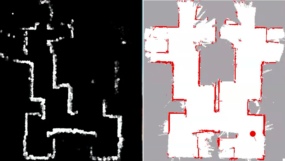
The easiest way for a robot to map its environment is using an occupancy grid. As the robot moves through its environment, the readings returned from its laser range finder (LRF) at different angles around it are marked off on a map. As a spot is marked more than once, its probability increases. This simulation shows the creation of an occupancy grid map. However, in the real world, odometry is not perfect and the robot’s position (as estimated by odometry) drifts from its real position, resulting in a skewed map. Hence, the requirement for a loop-closing technique like SLAM (Simultaneous Localization & Mapping) that corrects for this error when the robot doubles back on itself and visits a previously known location.

Occupancy Grid Simulation


See the simulation here:

Particle Filter Localization for a Simulated Mobile Robot

This entry is part 2 of 3 in the series Python Robotics Simulator

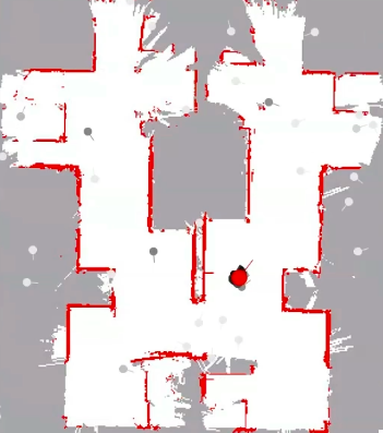
This simulation shows a robot (red) moving through a simulated environment and a Particle Filter (PF) trying to localize it in that environment. Initially, the particles (shown in different shades of grey indicating their probabilities) do not know the location of the robot and try and localize the robot from scratch. This is called global localization. After the robot moves about in its environment, the particles coalesce on the robot’s correct position. Thereafter, it is easier for the PF to track the position of the robot and this is called position tracking. Note that the environment is quite symmetric and this is why the PF has difficulty in finding the robot in the beginning, but gets there in the end.

Particle Filter Localization for a Simulated Mobile Robot


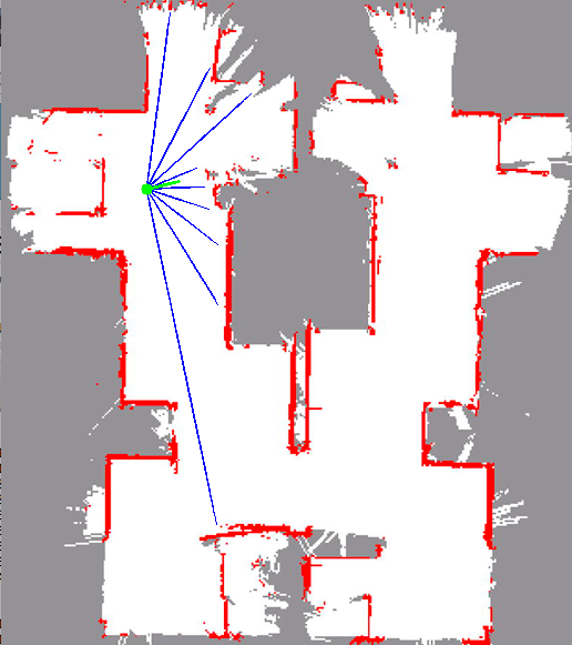
The measurements are simulated laser range finder readings (see previous post: Simulated Laser Range Finder Readings Using Python & OpenCV).
The code is written in Python using the OpenCV library (wrapper for python). It is adapted from PF code written by Juan Carlos Kuri Pinto and the Udacity team over at Udacity University’s online Autonomous Driving class (http://www.udacity-forums.com/cs373/questions/14131/unit-3-graphical-demo-of-ro­bot-localization-based-on-particle-filters).

See the video of the simulation here:

I’ll put the code up as soon as I’ve tidied it up a bit.

Setting up OpenCV 2.2 with Python on OS X

This post should be useful to Mac users who want to get OpenCV up and running with Python. I’ve recently migrated to an older (2010 refurbished) MacBook Air (from a 2011 MacBook Pro) which runs OS X 10.6.8 (The Pro ran 10.7.something). I transferred all my installed software from the Pro to the Air using Apple’s Migration Assistant software. However, after this, XCode (4.something) stopped working. I wasn’t able to install new stuff using MacPorts, and so I decided to uninstall XCode, uninstall MacPorts, install HomeBrew (instead of MacPorts to install Unix tools Mac didn’t ship with OS X) & install an older version of XCode (3.2.2). Python 2.6 was already installed and working fine. Here are the steps:

  • Uninstall MacPorts:
    • sudo port -f uninstall installed
    • sudo rm -rf /opt/local
      sudo rm -rf /Applications/DarwinPorts
      sudo rm -rf /Applications/MacPorts
      sudo rm -rf /Library/LaunchDaemons/org.macports.*
      sudo rm -rf /Library/Receipts/DarwinPorts*.pkg
      sudo rm -rf /Library/Receipts/MacPorts*.pkg
      sudo rm -rf /Library/StartupItems/DarwinPortsStartup
      sudo rm -rf /Library/Tcl/darwinports1.0
      sudo rm -rf /Library/Tcl/macports1.0
      sudo rm -rf ~/.macports
    • Remove /opt/local/bin & /opt/local/sbin from your PATH variable. To do this, open a new terminal window and type: open .profile. This will open up the .profile file using TextEdit (assumed installed). Comment out the line (prefix with #) the line: export PATH=/opt/local/bin:/opt/local/sbin:$PATH
  • Install HomeBrew: Open a terminal window and type:  /usr/bin/ruby -e “$(/usr/bin/curl -fksSL https://raw.github.com/mxcl/homebrew/master/Library/Contributions/install_homebrew.rb)”
  • Update HomeBrew: sudo brew update
  • Uninstall XCode 4.0 and install XCode 3.2.2:
    • Note: This step is not required if your XCode is running okay. You can diagnose this by:  sudo brew doctor
    • For example, I got the warning: Warning: You have no /usr/bin/cc.
      This means you probably can’t build *anything*. You need to install the Command Line Tools for Xcode.
    • So, uninstall XCode by:  sudo /Developer/Library/uninstall-devtools –mode=all
    • Download XCode 3.2.2 (without the iOS SDK, it is 745 MB) and install it the regular way (you get a .dmg file)
    • Now, typing gcc in the command line tells me that I have the following C/C++ compiler installed: i686-apple-darwin10-gcc-4.2.1
  • Install OpenCV 2.2: sudo brew install opencv –build32  (Note: –build32 because mine was a 32 bit OS). OpenCV installs in/Library/Frameworks/OpenCV.framework
  • Add Python Path: Open a new terminal and type open .profile and add this line: export PYTHONPATH=”/usr/local/lib/python2.6/site-packages:$PYTHONPATH”
  • Run OpenCV in Python:
    • Now, write the python program to do whatever you want. Import the OpenCV library by adding  import cv up the top of your program.
    • Now, to run a sample Load & Display Image program in python using the OpenCV library:

import cv

im = cv.LoadImageM("image.jpg")
cv.NamedWindow("loaded_image", 1)
cv.ShowImage("loaded_image",im)
cv.WaitKey(2000)

    • Note that there seems to be some bug with OS X and OpenCV with closing GUI windows. So I’ve used the cvWaitKey command above to automatically close the window after 2 seconds.
    • Sample face detection program (from http://recursive-design.com/blog/2010/12/14/face-detection-with-osx-and-python/ , remember to change the location of the Haar Cascade; mine was in /Library/Frameworks/OpenCV.framework/Versions/Current/Resources/) outputs:

Holographic HUD


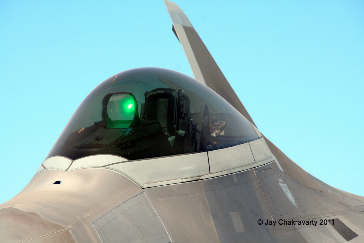
The holographic Heads Up Display (HUD) on the F-22 at this year’s Avalon Air Show. These HUDs use laser and computer-generated interference patterns to project light exactly where you want on the display and not elsewhere, leading to excellent readability in bright sunlight. Here’s a civilian version, by a UK-based company : http://lightblueoptics.com/products/light-speed/ that’s coming to a car near you.